
Abstract
Tolerance intervals are used to statistically derive the acceptance limits to which drugs must conform upon manufacture (release) and throughout shelf-life. The single measurement per lot in release data and repeated measurements per lot longitudinally for stability data have to be considered in the calculation. Methods for the one-way random effects model by Hoffman and Kringle (HK) for two-sided intervals and Hoffman (H) for one-sided limits are extended to a random-intercept, fixed-slope model in this paper. The performance of HK and H was evaluated via simulation by varying the following factors: (a) magnitude of stability trend over time, (b) sample size, (c) percentage of lot-to-lot contribution to total variation, (d) targeted proportion, and (e) data inclusion. The performance metrics are average width (for two-sided) or average limit (for one-sided) and attained confidence level. HK and H maintained nominal confidence levels as originally developed, but H is too conservative (i.e., achieved confidence level exceeds the nominal level) in some situations. The HK method adapted for an attribute that changes over time performed comparably to the more computationally intensive generalized pivotal quantity and Bayesian posterior predictive methods. Mathematical formulas and example calculations as implemented using R statistical software functions are provided to assist practitioners in implementing the methods. The calculations for the proposed approach can also be easily performed in a spreadsheet given basic regression output from a statistical software package. Microsoft Excel spreadsheets are available from the authors upon request.
LAY ABSTRACT: Tolerance intervals (a measure of what can be expected from the manufacturing process) calculated from attribute measurements of drug product lots are one of the factors considered when establishing acceptance limits to ensure drug product quality. The methods often used to calculate tolerance intervals when there are multiple measurements per lot and the attribute changes over time are either lacking in statistical rigor or statistically rigorous but computationally intensive to implement. The latter type requires simulations that have to be programmed using specialized statistical software, because closed-form mathematical formulas are not available. As a consequence, some quality practitioners and applied statisticians involved in setting acceptance limits may be hindered in using such computationally intensive methods. This paper aims to address this need by proposing an approach that is statistically rigorous yet simple enough to implement using spreadsheets. The approach builds upon previously published works developed for attributes that do not change over time and adapts the cited works for attributes that change over time. The proposed approach is demonstrated to have good statistical properties and compares favorably against the more computationally intensive alternative methods. The paper provides closed-form mathematical formulas, example data, and illustrative calculations as implemented in programmed R functions to facilitate implementation by practitioners. Alternatively, the calculations can be performed without requiring complex programming/simulation using Microsoft Excel spreadsheets that can be requested from the authors.
- Bayesian posterior predictive
- Generalized pivotal quantity
- Random effects model
- Release and shelf-life specification limits
- Tolerance interval
1. Introduction
Manufacturers set specification limits as part of an overall control strategy to ensure quality and consistency of their products. The regulatory guidance for setting specification limits for biological products ICH Q6B (1) defines specification for a quantitative quality attribute as the numerical limits to which a drug product or drug substance should conform to be considered acceptable for its intended use. Specification limits are further categorized into release and shelf-life limits. A product must meet release limits at the time of manufacture. A product must conform to shelf-life limits throughout its entire shelf-life (or expiration dating period). Release limits are normally more restrictive (i.e., narrower) than shelf-life limits to allow for uncertainty in degradation estimates to have a high assurance that the product will remain within the shelf-life limits. Release limits are either required to be formally registered with European health authorities or only serve as an internal control strategy for drug products marketed in the United States and Japan.
In the Six Sigma parlance, specification limits reflect the voice of the customers. The customers in the pharmaceutical industry are the patients, and the desired products are safe and efficacious drugs. Hence, specification limits of new drug products should ideally be the demonstrated ranges of quality attributes that assure clinical safety and efficacy. Often, the quantity of lots used for clinical studies are limited and do not reflect the full variability expected from the process. Per ICH Q6B (1), other factors such as relevant development data, pharmacopeial standards, and results from accelerated and long-term stability studies may be considered, as appropriate, to justify specification. The scope of this paper is the statistical derivation of specification limits based on analysis of quality attribute measurements taken at the time of manufacture (referred to as “release”) and over time for product stability assessment (referred to as “stability”). The shelf-life of the product is assumed to have already been established to avoid a circular exercise of setting both specification limits per ICH Q6B (1) and shelf-life per ICH Q1E (2) from the same stability data. If shelf-life also needs to be established, sponsors typically rely on nonstatistical considerations (e.g., business strategy, platform knowledge on a similar product) to inform their decisions. Alternatively, a shelf-life can be provisionally proposed. Then specification limits that will result in an acceptable out-of-specification rate given the observed data are calculated using the method described in this paper.
ICH Q6B (1) does not prescribe a particular statistical method to derive specification limits, but it recommends consideration of a reasonable range of expected analytical and manufacturing variability. Regulatory agencies typically leave it to drug sponsors to justify the basis of their proposed specification. The objective of this paper is to propose a closed-form tolerance interval-based method that accounts for random lot effect to statistically derive release and shelf-life specification limits. It will be shown that the proposed method performs satisfactorily per the defined metrics and comparably with the more complex modeling methods of generalized statistical intervals and Bayesian estimation. The proposed method is implemented via the R functions supplied in Appendix B, thus providing industry practitioners a tool for deriving specification limits. Alternatively, the calculations can be performed without requiring complex programming/simulation using Microsoft Excel spreadsheets that can be requested from the authors. Other approaches that had been published in the literature are first surveyed.
1.1. Survey of Methods for Setting Release and Shelf-Life Limits
Release limits are set such that if met at the time of manufacture, there will be a high assurance that the attribute will remain within the shelf-life limits throughout the expiry of the product. Hence, the two limits should be set jointly from both the release and stability data. The method by Allen et al. (3) has become the industry standard for setting release limits. Wei (4) proposed three alternative methods to improve Allen et al.'s (3) method, as the latter is characterized to lack statistical justification. Bayesian approaches also have been described by Shao and Chow (5), Manola (6), and Hartvig (7) for setting release limits. These aforementioned works do not address calculation of shelf-life limits and assume these limits already exist.
Because calculation of specification limits involves prediction of future values for a large proportion of units produced from the manufacturing process, an applicable statistical interval for this purpose is a tolerance interval (TI). Such a practice was suggested by Hahn and Meeker (8) and it appears in numerous other applications in the literature. The particular type of tolerance interval commonly used is the P-content interval, which is an interval that can be claimed to contain at least a proportion P of the population with a specified degree of confidence 100(1−α)%. If release limits are established on the basis of only release data (which typically have single measurement per lot), calculation of a tolerance interval with an independent sample of n values is straight-forward [for example, see Meeker et al. (9)]. However, release limits should not be set apart from shelf-life limits as previously mentioned. Rather, the two limits are ideally derived jointly from combined release and stability data to better inform estimates of variability. Calculation of tolerance intervals with repeated-measures data (as is the case with stability data) is more complicated than when there is only single measurement per lot because measurements on the same lot are not independent. Following ICH Q1A (10), stability data have repeated lot measurements corresponding to a fixed testing schedule—0, 3, 6, 9, 12, 18, 24, and 36 months. Because lots are enrolled in the stability study as manufactured, stability data are inherently unbalanced owing to the staggered ages of stability lots, creating more complexity in the data analysis.
The trend over time of a quality attribute in a stability study may be described in one of two ways. It either does not change over time (i.e., not stability-indicating) or changes over time (i.e., stability-indicating). Selection of the more appropriate trend assumption should not be based solely on a statistical test of significance on slope. Rather, scientific judgment based on the nature of the attribute and its expected stability-indicating behavior for the storage condition should also be considered. When an attribute does not change over time, the stability measurements for a lot can be assumed to be repeated measures for that lot. When there is process variability across lots, measurements within a lot are correlated, and the degree of correlation increases as the lot-to-lot variation increases. The statistical analysis must appropriately take this correlation into consideration. An appropriate statistical model for representing this correlation is the one-way random effects design. Calculation of a tolerance interval for a one-way random effects design has been widely studied for both balanced and unbalanced data [see chapters 4 and 5, respectively, of Krishnamoorthy and Mathew (11)]. The current paper uses the approach of Hoffman and Kringle (12) and Hoffman (13) to describe two-sided and one-sided tolerance limits, respectively, for both balanced and unbalanced data. These methods are hereafter referenced as HK and H in this paper.
When an attribute changes over time, the functional relationship between the attribute and time must be added to the one-way random effects model. In this paper, we assume the functional relationship is linear and the slope is constant across all lots. This model is justifiable from a process development perspective. Although intercepts that represent release values are expected to vary from lot to lot within some acceptable range, the rate of degradation over time (i.e., slope) is expected to be common or fixed among the lots for a well-characterized and sufficiently controlled manufacturing process. If the functional relationship of the stability-indicating attribute with time is not intrinsically linear (i.e., cannot be transformed or expressed as a polynomial), the HK and H methods described in this paper cannot be applied. Other methods such as the Bayesian posterior predictive method may be applicable. An applicable nonlinear likelihood model can be simply specified. A formal evaluation of methods that can handle a nonlinear functional relationship with time is outside the scope of the current paper.
There are some alternative methods to HK and H that can be used to construct tolerance intervals for the model of interest. Liao et al. (14) developed procedures for this purpose based on generalized pivotal quantities (GPQ). Bayesian simulation based on posterior predictive distribution of the parameters as applied to regression and hierarchical models [for example, see Wolfinger (15), Gelman and Hill (16), and Kruschke (17)] can also be used to calculate tolerance intervals. This is referred to as BayesPP in this paper. The hierarchical model when applied to the stability data simplifies to a one-way random effects design under the constant slope assumption.
1.2. Focus of the Current Work
Given our desire for a computationally simple approach, the work in this paper provides an in-depth study of the HK and H methods. The application to the non-stability-indicating trend is included for completeness. For the stability-indicating trend, the HK and H methods are modified for unbalanced data with incorporation of a fixed regression line using the results of Park and Burdick (18). The proposed approach posits that both release and shelf-life limits can be set by calculating tolerance limits from the release and stability data as evaluated at t0 = 0 and t0 = shelf-life, respectively, in the fitted regression model. The paper provides formulas for non-stability- and stability-indicating trends with application to an example data set. The performance of the proposed approach is then evaluated in a comprehensive simulation study across several conditions.
The GPQ and BayesPP methods are also implemented later in this paper for the stability-indicating trend albeit in a limited simulation study owing to the long computing times for these methods. The proposed HK and H methods are benchmarked against the more computationally complex GPQ and BayesPP methods to determine the performance loss (if any) for the simplified approach. It will be shown that the proposed simpler methods perform favorably relative to the more complex alternative methods.
2. Methodology
2.1. Proposed Approach (H and HK Methods)
When there are repeated measurements on some or all of the lots, the correlation among the values within a lot must be properly modeled to correctly calculate tolerance intervals. Hoffman and Kringle (12) and Hoffman (13) developed methods for two- and one-sided tolerance intervals, respectively, that can be used for non-stability-indicating methods with unequal numbers of repeated measures in each lot. These intervals are described below.
2.1.1. Attribute That Does Not Change with Time:
A quality attribute that does not change with time (i.e., is non-stability-indicating) is described using the following model:
 where Yij is the measured response for lot i at time j, μ is the overall mean, and Ai and Eij are independent normal random variables with zero means and variances σA2 and σE2, respectively. These assumptions imply that Yij is a normal random variable with mean μ and variance σA2 + σE2.
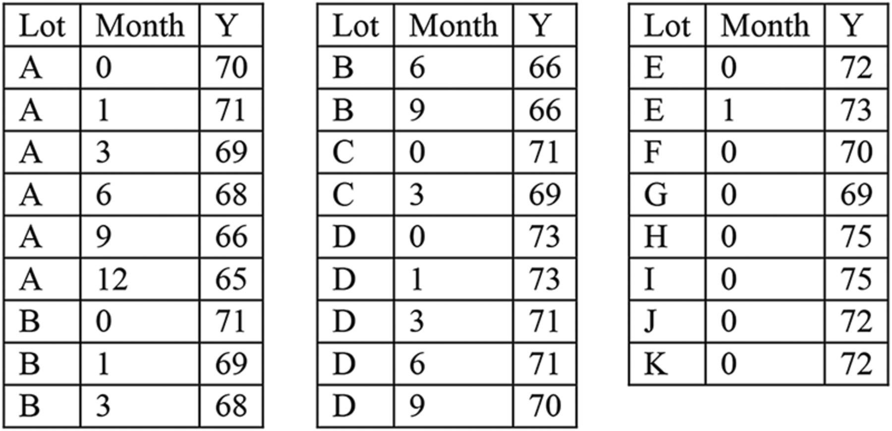
We now present tolerance interval formulas for an attribute that is non-stability-indicating. The notation is defined in Table I, with results of a numerical example included for the data shown in Appendix A. This data set contains both stability lots and lots with release values only. Note that the example data show a trend over time but can still be used to illustrate the calculations when assuming no trend.
Notation and Numerical Calculations for No Trend Over Time
The 100(1 − α)% lower tolerance bound that is less than at least 100P% of the population from Hoffman (13) is as follows:
 where Ȳ* is the unweighted sample mean of lot means, ZP and Z1−α are percentiles from the standard normal distribution with areas P and 1−α, respectively, to the left, and U is the 100(1−α)% upper bound on the total variance σA2 + σE2. Other notation is shown in Table I along with the results of a numerical example for the data included in Appendix A.
The 100(1−α)% upper tolerance bound that is greater than at least 100P% of the population from Hoffman (13) is:
Equations 2 and 3 are denoted as “H” in the simulation results that follow.
The 100(1−α)% two-sided tolerance interval that contains at least 100P% of the population from Hoffman and Kringle (12) is:
Equation 4 is denoted as “HK” in the simulation results that follow. The two-sided bounds in Equation 4 can also be used to construct one-sided intervals by replacing  with ZP. These one-sided intervals are referred to as “HK1” in the simulations.
2.1.2. Attribute That Changes with Time:
A quality attribute that changes with time (i.e., stability-indicating) is described using the following model:
 where all previous terms are as defined in eq 1, tij is the time point for the measurement taken on lot i at time j, and β is the fixed slope. These assumptions imply that Yij is a normal random variable with mean μ + βt0 and variance σA2 + σE2.
Hoffman (13) provides an example data set for the model in eq 5, but details are not provided to account for the fixed slope. Using results from Park and Burdick (18), we provide the required tolerance intervals based on both Hoffman and Kringle (12) and Hoffman (13). The one-sided 100(1 − α)% lower bound that is less than 100P% of the population is as follows:
 where Ŷ is the predicted value of Y at t0. The remaining terms have been defined in eq 2. Other notations are shown in Table II along with the results of a numerical example for the data included in Appendix A.
Notation and Numerical Calculations for With Trend Over Time
The computed one-sided upper 100(1 − α)% bound that exceeds 100P% of the population from Equation 1 of Hoffman (13) is:
The two-sided 1 − α tolerance interval that contains 100P% of the population from Hoffman and Kringle (12) is:
The point estimator for β in the first row of Table II is obtained by regressing Y on tij and lot in a fixed-effect model. The term SE2 is the mean squared error for this model. The two-sided bounds in eq 8 also can be used to construct one-sided intervals by replacing  with ZP. These one-sided intervals are referred to as “HK1” in the simulations.
2.2. Simulation Study Design
The performance of the intervals described above is evaluated in a simulation study. Factors studied are described in Table III. The intraclass correlation is defined as ρ = σA2/(σA2 + σE2) and represents the correlation among measurements in the same lot. Without loss of generality, σA2 = ρ, σE2 = 1 − ρ and μ = 100 are used in the simulation study. The nominal confidence coefficient was 95% for all cases.
Study Design Levels Used in Simulation
2.3. Simulation Performance Metrics
For an attribute that does not change with time, the first performance metric is the average width of the calculated two-sided tolerance intervals normalized by the width of the true specification limits, 2 × Z(1 + P)/2  . The closer the average normalized width is to 1 without dropping below, the better is the method. For one-sided limits, the average upper and lower bounds are normalized by their true one-sided upper and lower specification bounds, respectively. For upper bounds, it is desirable to be as close to 1 as possible without dropping to less than 1, and for lower bounds, it is desirable to be as close to 1 as possible without becoming greater than 1. For an attribute that changes with time, the limits of interest are lower release limits (LRL) evaluated at t0 = 0 and lower shelf-life specification limits (LSL) evaluated at t0 = shelf-life.
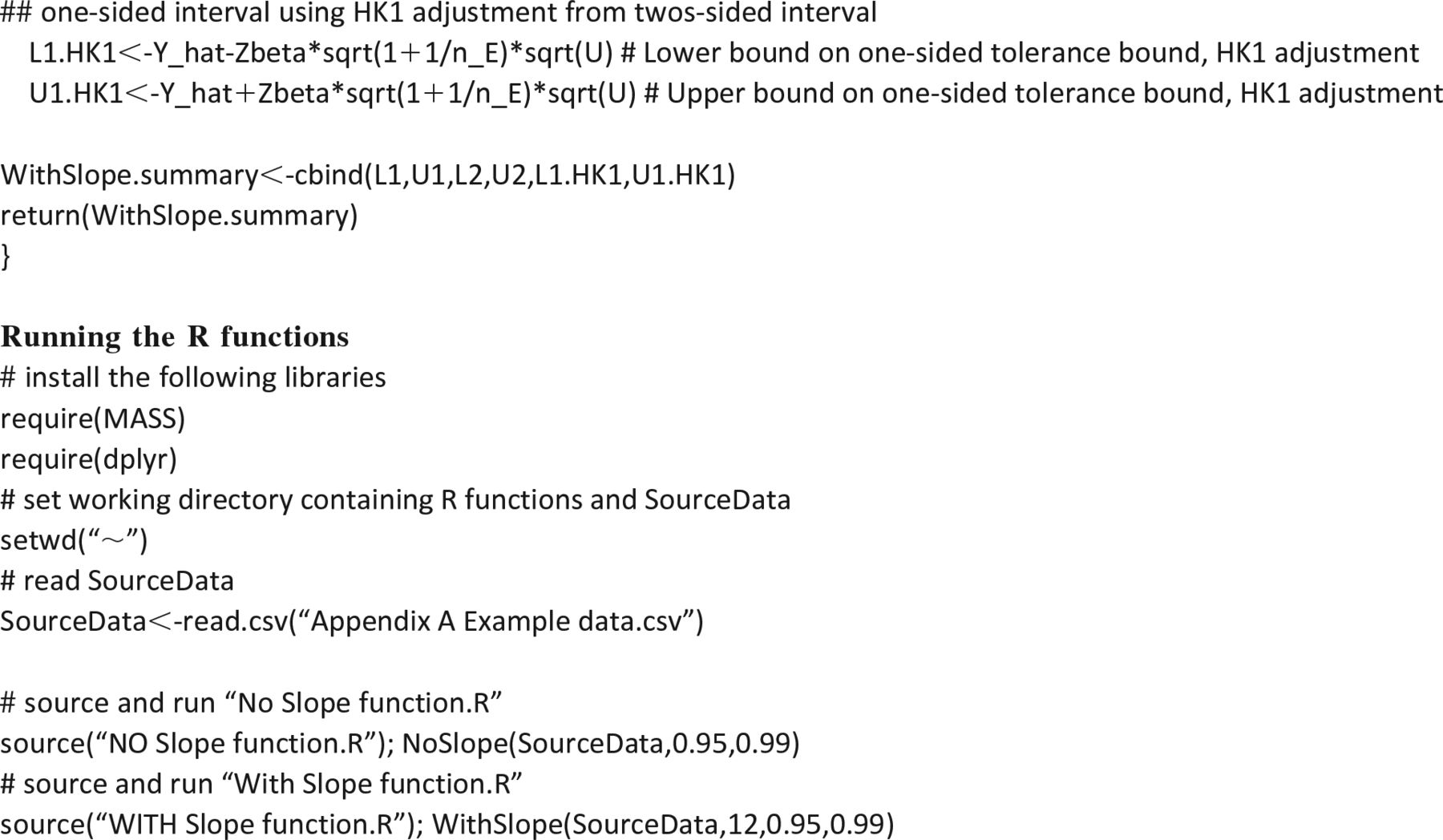
The second performance metric is the confidence coefficient, which is the fraction of the total simulation iterations where the calculated two-sided tolerance interval contained the targeted proportion (for two-sided limits) or the calculated one-sided bound correctly bracketed the true one-sided bound (for each of the one-sided lower and upper limits). The closer the confidence coefficient is to the nominal level without dropping below it, the better is the method. Each simulation is based on 10,000 iterations. Thus, if the true confidence coefficient is 0.95, the binomial approximation defines the 95% simulation error to be 1.96  = 0.004. This means that if the true confidence coefficient is 95%, we expect to see the simulated confidence coefficient in the range of 94.6% to 95.4%. Although shorter average normalized widths or limits are preferable, it is necessary that a method first maintain the stated confidence level. All analyses are performed using R 3.2.2 statistical software (19). Programmed R functions for non-stability-indicating and for stability-indicating attributes are included in Appendix B, which readers can implement in their own data. For practitioners that do not use the R programming language, the formulas presented in Table I and Table II are implemented in Microsoft Excel spreadsheets and are available from the authors upon request.
2.4. Alternative Approaches (GPQ and BayesPP)
2.4.1. Generalized Pivotal Quantity:
Tsui and Weerahandi (20) introduced the concept of generalized inference for testing hypotheses when exact methods do not exist. Weerahandi (21) extended this concept to construct generalized confidence intervals (GCIs). Hannig et al. (22) have shown that under very mild conditions, these intervals provide correct frequentist coverage. That is, for practical purposes, they can be considered “calibrated.”
A tolerance interval can likewise be formulated using this approach. In particular, Liao et al. (14) provide an algorithm in Section 5 of their paper that can be used to form both one- and two-sided P-content tolerance intervals for the stability model considered in this paper (see Section 5.4 of their paper for an illustrative example). This process can be time-consuming on a computer, because it requires a simulation-based solution with the need to solve a nonlinear equation on each iteration. The tolerance interval is computed based on the sample percentiles of the resulting set of simulation realizations.
The GPQ algorithm in Liao et al. (14) is applied to an attribute that decreases over time in this paper. Tolerance bounds derived from a selected percentile (i.e., 100% − 99.73% = 0.27% for proportion P = 0.9973) of 10,000 simulation realizations evaluated at t0 = 0 and t0 = shelf-life are designated as one-sided LRL and LSL, respectively. The method is implemented using SAS/IML 14.1 (23).
2.4.2. Bayesian Posterior Predictive:
Bayesian simulation based on posterior predictive distribution of the parameters as applied to regression and hierarchical models [for example, see Wolfinger (15), Gelman and Hill (16), and Kruschke (17)] is used to calculate tolerance intervals in this paper. For an attribute that changes over time, the random-intercept, fixed-slope model previously shown in eq 5 is used as the data likelihood model. This model is presented again in eq 9 along with the noninformative priors used for the model parameters μ, Ai, β, and Eij.
JAGS version 4.3.0 is used to produce a 20,000-draw sample from the posterior distribution of model parameters using Markov-chain Monte Carlo (MCMC) simulation. Future predicted values evaluated at both t0 = 0 and t0 = shelf-life are generated from the drawn posterior samples of the model parameters. The tolerance limits derived from the specified percentile (i.e., 100% − 99.73% = 0.27% for proportion P = 0.9973) of the posterior predictive distributions at t0 = 0 and t0 = shelf-life are designated as one-sided LRL and LSL, respectively. Note that the tolerance limits calculated using the BayesPP method in this paper are of the P expectation type (i.e., limit that contains a proportion P of the population, on the average). On the other hand, tolerance limits calculated using H, HK1, and GPQ methods are of the P-content type (i.e., limit that can be claimed to contain at least a proportion P of the population with a specified degree of confidence) (11).
If a random-intercept, random-slope model is more appropriate for the attribute of interest, the Bayesian estimation procedure described above is modified by using the corresponding model in eq 10. The noninformative priors related to the random slopes βi are also shown in eq 10. The priors for the rest of the model parameters are the same as in eq 9.

The BayesPP method is implemented in this paper using R 3.2.2 statistical software (19) with “runjags” (24) and “rjags” (25) library packages to use JAGS as the MCMC algorithm. Detailed implementation of JAGS for a hierarchical model is presented in Chapter 17, Section 3 of Kruschke (17).
3. Results and Discussion
3.1. Comprehensive Evaluation of the HK and H Methods
The results of the comprehensive simulation study as designed in Table III are first presented. The performance metrics are plotted versus the targeted proportion (P) on the x-axis with column stratification by sample size and intraclass correlation coefficient (ρ, rho) and a grouping variable derived from concatenating the data used (RS = combined release and stability data; S = stability data only) and the method applied [HK (12); H (13)]. For example, the concatenated grouping RS_HK means release and stability data were combined and analyzed with the HK method (12). Where the HK method was modified to apply to one-sided limits, the method is notated as HK1. The metrics for performance evaluation are graphically summarized in Figure 1 through Figure 4.

Normalized average widths (left) and confidence coefficients (right) for no change with time, two-sided limits.
Note: Red-dashed reference line is the target value for the metric.
Figure 1 displays the results for the two-sided HK method for no change with time. The combined release and stability (RS) data provide narrower normalized averaged widths than using only stability (S) data. The RS confidence coefficients are satisfactory except in the large sample size design with ρ = 0.2. In this case, the simulated confidence coefficient falls slightly below the nominal level.
Figure 2 displays results for the one-sided H and HK1 methods where there is no change with time. The normalized average lower and upper limits are shown in a single plot. The RS_HK1 and S_H results are closest and farthest, respectively, from the true limits. The confidence coefficients are approximately the same for lower and upper limits, so only the one-sided lower limits are presented. The H method confidence coefficients are well above the nominal level and are too conservative. This is consistent with the results in Hoffman (13) where the author used a boot-strapping approach to bring the confidence coefficients closer to the nominal level to make the method less conservative. We wanted to investigate the possibility of expressing the HK two-sided limits as one-sided limits for this case (HK1). The RS_HK1 confidence coefficients fall significantly below the nominal level when the value of P is less than 0.99. However, for the values of P equal to 0.99 and 0.9973, the simulated levels are reasonably close to the nominal level and preferred over the very conservative H intervals.

Normalized average lower and upper limits (left) and confidence coefficient for lower limits onlya (right) for no change with time, one-sided limits.
Note: aOnly confidence coefficients for lower limits are shown, as upper limits follow the same trend as lower limits. Red-dashed reference line is the target value for the metric.
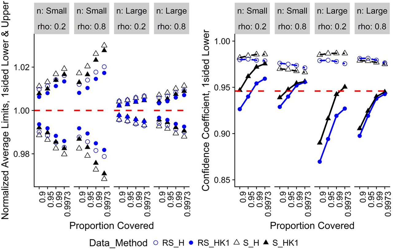
For change with time, the specific simulated trend was for an attribute that decreases over time β = −0.15. Therefore, the limits of interest to drug sponsors are one-sided LRL and one-sided LSL. If an increasing trend is expected, one-sided upper limits are calculated instead of lower limits. Figure 3 displays one-sided H and HK1 LRL results. The normalized average LRL for RS_HK1 and S_H are closest and farthest, respectively, from the true limits. The H confidence coefficients are well above the nominal level with some improvement depending on whether S or RS data were used. The RS_HK1 confidence coefficients are below the nominal level at low target proportions but improve as target proportion increases. S_HK1 has better confidence coefficients than RS_HK1. Figure 4 displays one-sided H and HK1 LSL results, where the relative performances of the methods are approximately the same as for the one-sided LRL (Figure 3). This is an expected outcome of the holistic approach of using the same method applied to both limits. The only difference is the time point at which tolerance bounds are calculated, i.e., to = 0 and to = expiry for release and specification limits, respectively. It can be shown that the distribution of the difference between release and shelf-life limits in the 10,000 iterations centers around average change over the shelf-life, β × texpiry with some randomness due to process, sampling, and analytical variability.

Normalized average limits (left) and confidence coefficients (right) for change with time, one-sided lower release limits (t0 = 0).
Note: Red-dashed reference line is the target value for the metric.

Normalized average limits (left) and confidence coefficients (right) for change with time, one-sided lower specification limits (t0 = shelf-life).
Note: Red-dashed reference line is the target value for the metric.
3.2. Benchmark Comparison of HK1 and H Methods Versus GPQ and BayesPP
Next, we investigated whether the simplified HK1 and H methods have any performance loss by benchmarking against GPQ and BayesPP methods. The latter two methods derive limits by simulating future values per iteration as described in the Methodology. Table IV contrasts the number of simulated future values per iteration for GPQ (i.e., 10,000) and BayesPP (i.e., 20,000) versus the proposed approach (i.e., no simulation required because closed formulas are used). This underscores how much more computationally intensive GPQ and BayesPP are than the H, HK, and HK1 methods. Because it is not feasible to evaluate GPQ and BayesPP methods in a 10,000-iteration simulation study, a limited 100-iteration simulation study is instead used for benchmarking the proposed approach. The relative trends among the compared methods should already manifest in 100 iterations; hence, the limited simulation is fit for the purpose of benchmarking. The scenario selected from Table III for this limited simulation study is β = −0.15, ρ = 0.8, P = 0.9973, RS (combined release and stability data) with both small and large sample sizes. Because there is a negative trend over time, one-sided LRL and one-sided LSL are of interest. The HK method modified for one-sided, i.e., HK1, together with the H method are compared versus GPQ and BayesPP.
Computational Requirements in Simulation Studies
Recall that the slope was assumed fixed among the lots, as rationalized in the Introduction, so a random-intercept, fixed-slope model applies. This simplifying model assumption enables the derivations of the HK1 and H tolerance interval formula for stability-indicating attributes (Table II) and implementation of the GPQ method. If a random-intercept, random-slope model is instead more appropriate, modification of the H, HK1, and GPQ methods is nontrivial and is outside the scope of this paper. However, the Bayesian framework can easily incorporate the random effect of the lots in both intercept and slope. Therefore, the BayesPP is implemented using both fixed and random slopes in the limited simulation.
Before presenting the results of comparison of the frequentist approach (H, HK1, and GPQ) versus the BayesPP approach, it is important to point out the distinction between the two approaches. The tolerance intervals derived from the frequentist approach are calibrated to target achieving the nominal confidence under repeated sampling. On the other hand, the tolerance interval derived from BayesPP is conditioned on the observed data, and the confidence properties depend on chosen priors and are not expected to provide nominal frequentist confidence in general. Another way to frame the distinction is that the H, HK1, and GPQ tolerance intervals are P-content type, whereas that of BayesPP is a P-expectation type. The former is usually wider than the latter. Although the frequentist and Bayesian approaches are conceptually different, comparison of H, HK1, and GPQ to BayesPP is still useful. The results of the comparison are interpreted in the context of these differences.
Figure 5 presents overlay plots of the calculated LRL and LSL for small and large sample sizes, while Table V summarizes the performance metrics for the compared methods. As expected, all methods perform better as sample size becomes larger. HK1 and GPQ limits almost overlap each other. Both HK1 and GPQ methods maintain the nominal 0.95 confidence while very closely approximating the true limits. Note that had we selected P < 0.99, the HK1 would not have performed as well (refer to Figure 4 and Figure 5). The H method has slightly wider limits and is therefore more conservative than HK1 and GPQ. This observed trend is expected based on the findings from the comprehensive simulation. The BayesPP (random slope) generates a non-zero posterior predictive distribution of random slope variance, whereas the data it was conditioned upon were generated using zero-slope variance (fixed slope). As a consequence, the BayesPP (random slope) limits are too conservative. The BayesPP (fixed slope), although reflecting the zero-slope variance of the data it was conditioned upon, still falls below the 0.95 confidence. This is attributed to the P-expectation type of the BayesPP tolerance interval, whereas the H, HK1, and GPQ tolerance intervals are the P-content type.

Overlay plot of calculated one-sided lower release and shelf-life limits of proposed methods (H and HK1) versus GPQ and BayesPP methods for 25a iterations.
Notes: aOnly the first 25 of the calculated limits from the 100 iterations are shown to better visualize the relative trends. Evaluation of performance metrics summarized in Table V is based on all 100 iterations. BayesPP method expanded to include both cases when slope is treated as fixed and as random effect. For large sample (right panel), GPQ lines are overlapping with HK1 and therefore not visible. (red dashed lines) – true release and shelf limits.
Performance Metrics for Comparison of H and HK1 Versus GPQ and BayesPP
Overall, it is demonstrated that the computationally simpler HK1 method is comparable to the computationally more involved GPQ. The HK1 method provides more nominal coverage than the BayesPP method. Although not explored in the limited simulation, it can be inferred from the comprehensive simulation that when P < 0.99, the H method will be a better alternative to the GPQ and BayesPP methods than the HK1 method.
4. Summary and Recommendation
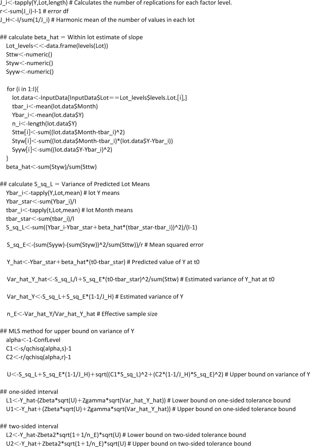
The one-way random effects model for two-sided tolerance intervals by Hoffman and Kringle (12) and one-sided tolerance limits by Hoffman (13) were extended to the mixed-effects linear regression with random intercepts and a fixed slope. This model is generally applicable to the type of stability data encountered in pharmaceutical manufacturing. The results are presented in a closed form to facilitate implementation of the method. The mathematical formulas are illustrated via a numerical example with R functions provided in Appendix B. As an alternative for users not programming in R statistical software, Microsoft Excel spreadsheets to perform all calculations are available from the authors.
The methods vary in performance depending on the intraclass correlation coefficient, sample size, targeted proportion, and whether release and stability data are combined. The studied methods are shown to have realized confidence coefficients close to the nominal confidence levels, although the one-sided limits of Hoffman (13) are perhaps too conservative. If covering proportions 0.99 or greater, one is better off using the individual one-sided bound of Hoffman and Kringle (12). Generally, combining both release and stability data will improve the precision and confidence coefficients. As expected, larger samples decrease the expected width of the tolerance interval. The proposed approach in this paper is relatively simpler to implement without any performance loss compared to more complex alternative methods. If a random-intercept, fixed-slope model cannot be justified for the attribute of interest, the proposed approach as currently formulated has limited applicability and can be a future area of research. The BayesPP method, although more computationally involved than the proposed approach, is versatile to handle the more complex random-intercept, random-slope model. In addition, historical knowledge on any of the model parameters can be specified into the priors of the Bayesian model for a scientifically driven estimation.
The formulas used require selection of an applicable stability trend for the attribute. The nature of the attribute and/or the condition under which the drug product is stored should inform this trend selection process. If the trend over time has to be inferred solely from the observed stability data, caution is advised, especially if there are limited stability time points. Incorrect selection of the non-stability-indicating formula when there truly is a trend will underestimate shelf-life limits, increasing the likelihood of getting out-of-specification batches and product recalls. On the other hand, selecting the stability-indicating formula when there truly is no trend will result in unrealistically low (or high) limits, especially if product shelf-life is long. It is good practice to have at least several stability lots with real-time measurements up to the expiry to increase the reliability of inferred trend over time.
Overall, the methods described provide a unified approach to statistically derive release limits and shelf-life specification limits using the same equation to calculate tolerance intervals of a random-intercept, fixed-slope model. This holistic approach implements the intent of the two-tiered control strategy of setting a release limit such that if a manufactured drug product lot meets it, the probability of exceeding the set specification limits during its shelf-life is reduced. The computed tolerance intervals described in this paper are only one consideration in setting product release limits and shelf-life specifications. The determination of the final product acceptance criteria should be jointly decided between the drug product developers (engineers, chemists, and biologists), clinicians, and statisticians using the statistically derived limits as a starting point, which are then weighed against process, analytical, and safety considerations.
Conflict of Interest Declaration
The authors declare that they have no competing interests.
Acknowledgments
The authors thank Jorge Quiroz (Merck), as well as the two reviewers for helpful suggestions to improve the manuscript.

Appendix: B


- © PDA, Inc. 2019


