
Abstract
Color is an important quality attribute for biotherapeutics. In the biotechnology industry, a visual method is most commonly utilized for color characterization of liquid drug protein solutions. The color testing method is used for both batch release and on stability testing for quality control. Using that method, an analyst visually determines the color of the sample by choosing the closest matching European Pharmacopeia reference color solution. The requirement to judge the best match makes it a subjective method. Furthermore, the visual method does not capture data on hue or chroma that would allow for improved product characterization and the ability to detect subtle differences between samples. To overcome these challenges, we describe a quantitative method for color determination that greatly reduces the variability in measuring color and allows for a more precise understanding of color differences. Following color industry standards established by International Commission on Illumination, this method converts a protein solution's visible absorption spectra to L*a*b* color space. Color matching is achieved within the L*a*b* color space, a practice that is already widely used in other industries. The work performed here is to facilitate the adoption and transition for the traditional visual assessment method to a quantitative spectral method. We describe here the algorithm used such that the quantitative spectral method correlates with the currently used visual method. In addition, we provide the L*a*b* values for the European Pharmacopeia reference color solutions required for the quantitative method. We have determined these L*a*b* values by gravimetrically preparing and measuring multiple lots of the reference color solutions. We demonstrate that the visual assessment and the quantitative spectral method are comparable using both low- and high-concentration antibody solutions and solutions with varying turbidity.
LAY ABSTRACT: In the biotechnology industry, a visual assessment is the most commonly used method for color characterization, batch release, and stability testing of liquid protein drug solutions. Using this method, an analyst visually determines the color of the sample by choosing the closest match to a standard color series. This visual method can be subjective because it requires an analyst to make a judgment of the best match of color of the sample to the standard color series, and it does not capture data on hue and chroma that would allow for improved product characterization and the ability to detect subtle differences between samples. To overcome these challenges, we developed a quantitative spectral method for color determination that greatly reduces the variability in measuring color and allows for a more precise understanding of color differences. The details of the spectral quantitative method are described. A comparison between the visual assessment method and spectral quantitative method is presented. This study supports the transition to a quantitative spectral method from the visual assessment method for quality testing of protein solutions.
Introduction
Color is a critical quality attribute for therapeutic proteins as defined in the International Conference of Harmonization (ICH) guidelines for biotechnological/biological products (ICH guideline Q6B) (1). There are numerous reports in the literature on the investigation of the causes of color in protein solutions such as photooxidation and co-eluting impurities (2⇓⇓–5). It is measured upon drug substance and drug product release, and during stability testing. Pharmacopeias related to protein solution biotherapeutics specify the method to characterize color (6). Currently, the standard practice utilizes a visual assessment method for characterizing a protein solution as well as for batch release/stability testing. In the visual assessment method, following preparation of a set of reference color solutions, an analyst visually compares a protein solution's color to that of the reference color solutions. Based on hue and intensity of the sample, as compared with the reference colors, the analyst reports the test result as one of the reference colors that most closely matches the sample. Preparing the reference color solutions requires mixing various amounts of components and liquid and hence introduces one possible source of variability. In addition, the color of the protein solution often resides somewhere in between the reference colors, and therefore an analyst is required to make the subjective visual judgment to determine the reference color that most closely matches the color of the sample.
An instrument-based quantitative method is preferred, as it removes both of these sources of variability. Such a method would eliminate the need to prepare reference color solutions, and the subjectivity of choosing the correct color series would be replaced with an algorithm. In addition, an instrument-based method would allow for greater granularity as compared with the visual method, and hence a greater degree of precision in the characterization of a protein solution's color. Here, we describe the development of a quantitative color measurement method that correlates to the currently used visual assessment method using the International Commission on Illumination (CIE)-defined L*a*b space as described in further detail in the Results and Discussion section.
Materials and Methods
Preparation of the European Pharmacopoeia (Ph. Eur.) Reference Color Solutions
Reference color solutions were prepared as described in Ph. Eur. 8.0 (6). In general, preparing the reference color solutions requires three steps: (1) dissolve the salt in 1% HCl solution to produce three primary color solutions, (2) primary color solutions are mixed in various ratios and diluted in 1% HCl to generate five standard color solutions, (3) each standard color solution is then further diluted with various amounts of 1% HCl to make the 37 reference color solutions.
For this study, we purchased the primary color solutions from Ricca Chemical Company (Arlington, TX). The blue primary color solution containing cupric sulfate was tested to contain 62.40 mg CuSO4.5H2O within the specification of 62.40 ± 0.04 mg/mL per the vendor's certificate of analysis (COA). The red primary color solution containing cobaltous chloride was tested to contain 59.52 mg/mL CoCl2.6H2O within the specification of 59.50 ± 0.02 mg/mL per the vendor's COA. The yellow primary color solution containing ferric chloride was tested to contain 45.02 mg/mL FeCl3.6H2O within the specification of 45.00 ± 0.03 mg/mL per the vendor's COA.
Typically, blue, red, and yellow primary color solutions would be mixed with 1% HCl volumetrically at different ratios (Table I) to generate the five Ph. Eur. standard color solutions: red (R), brown (B), brown yellow (BY), yellow (Y), and green yellow (GY). Then, the five color standard solutions are typically further diluted with 1% HCl volumetrically to make the complete set of reference color solutions (Table II). However, in this study, a gravimetric method was used as it is more accurate and precise than the volumetric method. The densities of each primary color solution and the 1% HCl were measured, and then the volumes (mL) of each composition in Table II were converted to the weight (g) (Table III). Density values are the average of three measurements performed using an Anton PAAR Digital Density Meter. The volumes of the standard color solutions in preparation of reference color solutions in Table IV were also converted to weights using the densities of the standard color solutions gravimetrically made from Table II (Table III). A calibrated analytical balance was used to weigh each of the composition reagents based on Tables II and III to make the 37 Ph. Eur. reference color solutions.
Preparation Ph. Eur. Standard Color Series Solutions (Volumetric Preparation)
Preparation of Ph. Eur. Reference Color Solutions (Volumetric Preparation)
Preparation of Ph. Eur. Standard Color Solutions (Gravimetric Preparation)
Preparation of Ph. Eur. Reference Color Solutions (Gravimetric Preparation)
Statistical Evaluation of Reference Color Solutions
For each of the five standard color solutions, multiple sets of independent batches were made. Then, for each batch of standard color solution, the full set of reference color solutions in that color series was prepared gravimetrically. Using a HunterLab UltraScan VIS (HunterLab Inc., Reston, VA), the color of each of the reference color solutions in the International Commission on Illumination (CIE) L*a*b* color space was measured five times, one time each by each of five different analysts.
The target L*a*b* values for a specific reference color solution were obtained by averaging the individual L*a*b* values obtained across batches and analysts. The method of moments was used to obtain estimates of the covariance matrices associated with the sources of variation due to batch-to-batch preparation, analyst-to-analyst variation, and instrument variability. A weighted sum of these individual covariance matrices provided an estimate of the total system covariance.
A 99% confidence region was obtained for the target L*a*b* value by assuming that the individual measurements followed a multivariate normal distribution. Assuming this statistical model, 100,000 random L*a*b* values were simulated. The smallest δ was determined such that the CIE ΔE2000 distance (see Results and Discussion section for description of ΔE2000) between 99% of the simulated values and the target value were no greater than δ. For all reference color solutions, the corresponding δ was less than 0.5, which is considered less than a visually observable difference in color, which is generally considered to be 1 for a small but perceptible difference in color (7). Thus, the confidence level is 99% that there is no visually observable difference in color between the target L*a*b* value and the true L*a*b* for all of the reference color solutions.
Interpolation of Points between Reference Color Solutions within L*a*b
Points between reference color solutions within a given series were interpolated using a spline function (MATLAB, Mathworks). Briefly the spline function uses a cubic spline interpolation to find yy (the interpolated L*a*b* values) from the underlying function Y (the standard L*a*b* values) at the values of the interpolant xx (arbitrarily defined by us as 10 points from one L*a*b* reference solution to another within a series). This was performed for each color series starting at water, so values are interpolated between water and the least-colored standard in a series as well as between every standard in a series. Appendix Table S3 shows the L*a*b* values of both the reference color solutions and the interpolated points.
Absorption Measurements and L*a*b* Transformation
All measurements were completed using a HunterLab UltraScan VIS spectrophotometer, which is a visible-range color measurement spectrophotometer that measures a sample's spectrum and correlates the physical spectral measurement to human color perception, which is a complicated process of photo-receptor activation and neurological processing. The instrument was standardized for 100% transmission (cuvette filled with water) and 0% transmission (light path blocked). All measurements were carried out using a 1 cm path length cuvette and the HunterLab micro cell holder. The system includes a spectrophotometer coupled to EasyMatchQC-ER software. In the UltraScan VIS optical system, the diffuse (sphere) geometry is configured for measurements in the total transmission (TTRAN) mode. The optical system has an effective bandwidth of 10 nm, and spectral data is collected every 10 nm. The conversion from absorption spectrum to color perception involves tristimulus color calculations, which are performed from 360 to 780 nm as recommended by the CIE (8). The software uses CIE L*a*b* values to represent different colors under daylight D65 and 10° standard observer conditions.
Visual Assessment
A light box with a diffuse fluorescent light source positioned in an inspection station with white background was used for the visual assessment method. The test tubes for the visual assessment method were clear, colorless, 12 mm outer diameter, borosilicate, flat-bottom tubes from VWR Scientific Products (Radnor, PA). For the visual assessment, the analyst looks down the long path length of the test sample (40 mm) following Ph. Eur. 2.2.2. test method 2; however, the data supplied here presumably will apply equally well to test method 1 (6) where the analyst views across the shorter path length of the sample. In either case, the analyst then picks the closest Ph. Eur. color series and reports the result as less than the next darker reference color in the best match color series. In this study all analysts used the same light box with the same light source in the same laboratory to minimize variation in perception of color due to factors such as light quality (light source temperature) and intensity.
Results and Discussion
The visible region of the electromagnetic spectrum falls between 360 and 780 nm. Light radiation in this region of the spectrum selectively excites one of three color receptors (cones) in the human eye, followed by neuro-processing and the resulting perception of color. When viewed against a white background, a protein solution will appear colored if there is a relative loss of radiation from part of the visible spectrum. For example, when blue light is absorbed the solution appears yellow. The selective loss of visible light passing through a protein solution can be caused by light scattering and/or from the absorption by chromophores. Although it is difficult to differentiate the contribution of scattering and chromophores to a drug product's overall color, it is nonetheless important to measure the color in a reproducible and accurate manner.
Because loss of light passing through a protein solution is the source of a protein solution's color, information about a solution's color is contained in its absorption spectrum. Differences in color can be quantified by converting to a scale that correlates to color perception. The conversion of an absorption spectrum to color perception employs a well-established methodology. We briefly outline the procedure here, but this topic is discussed in greater detail in the literature (8–9).
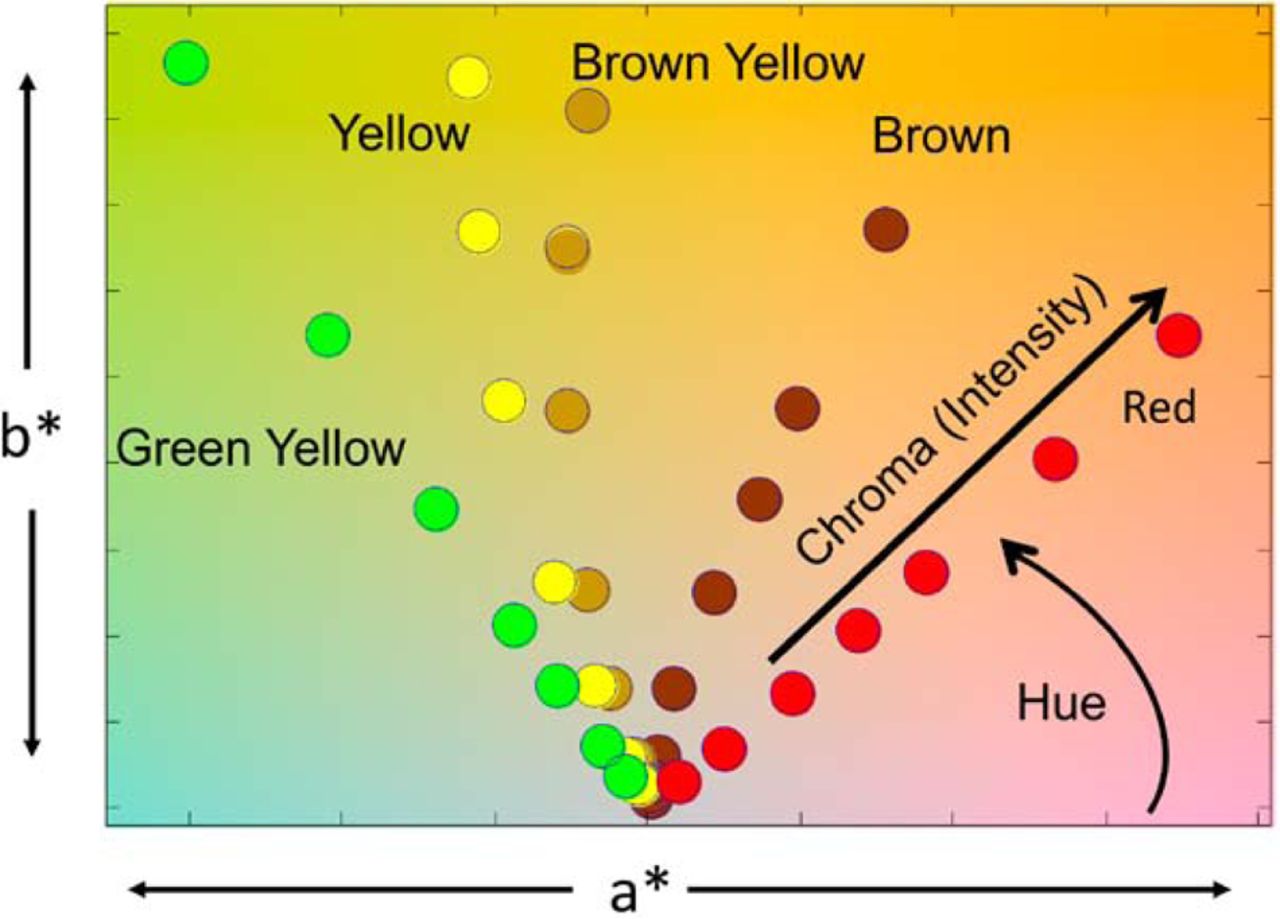
Differences in color perception can be quantified using the CIE standard system of color measurement (8–9). Briefly, the transmission spectrum is integrated into relative amounts of blue, green, and red light (8–9). These blue, green, and red values (expressed as Z, Y, and X, respectively, in the literature and referred to as tristimulus values (8) are then transformed into the L*a*b* color space (8–9). L*a*b* is a three-dimensional color space in which information about chroma (intensity) and hue are contained within the a*b* plane, and information about the relative lightness of the color is captured in the L* dimension. L* spans from 100, which is the equivalent of 100% light transmission/white, to 0, which is the equivalent of no light transmission/black. Within the a*b* plane, the horizontal a* axis spans from positive a* being red to negative a* being green; 0 is neutral. The vertical b* axis spans from positive b* being yellow to negative b* being blue, again with 0 being neutral.
Uniquely, the L*a*b* color space corresponds to a uniform spacing in visual perception. Therefore, the L*a*b* color space is able to quantify visual perception; two colors with a large color difference will have larger distance between their corresponding coordinates in L*a*b* space as compared with two colors that are closer in color.
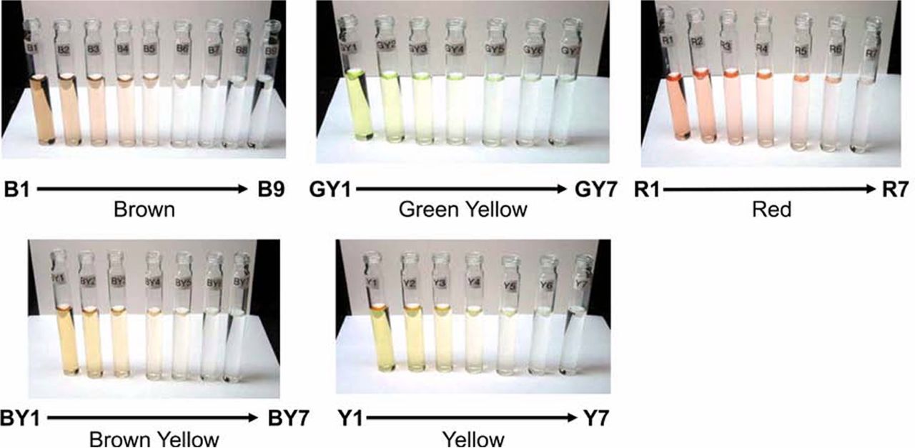
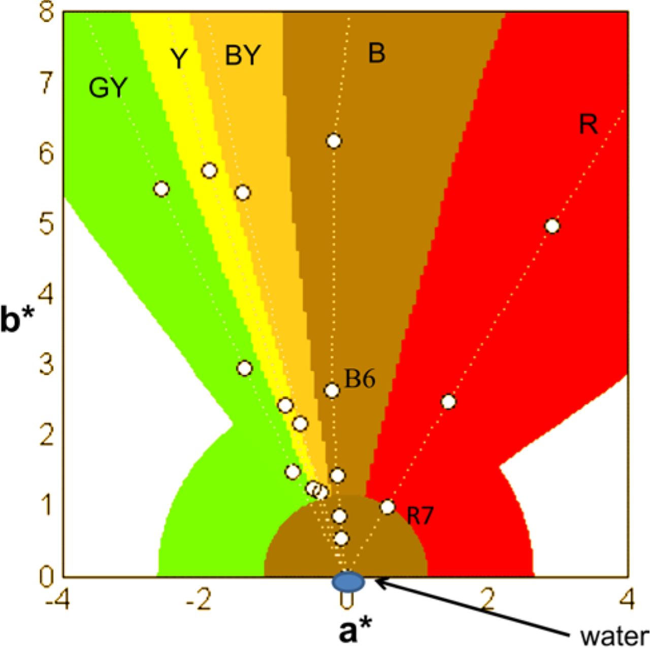
The Ph. Eur. reference color solutions used for visual assessment extend from red to greenish yellow (Figure 1). Figure 2 shows the 37 Ph. Eur. reference colors (Table I) as they appear within the a*b* plane with water (a*,b* = 0,0) included as a reference. These data were generated by taking the absorption spectra of all 37 reference color solutions and then calculating their corresponding L*a*b* values. It should be noted that for simplicity, the plots are represented in the a*b* space, but all calculations are performed using three-dimensional space. Within the L*a*b* color space, one can quantify hue and chroma. Hue is defined as the angle between a* and b*, and chroma is the radial distance from water (a*,b* =0,0). The Euclidean distance between two points plotted in the L*a*b* color space correlates to visual perception. As such, a larger Euclidean distance between two points in L*a*b* corresponds to larger perceived differences in color. As expected, water has no absorption in the visible region of the spectrum and appears at a* and b* equal to zero. The plots match our perception as the most dilute reference color solutions (R7, B9, BY7, Y7, and GY7) appear close to water, and the most intensely colored reference color solutions (R1, B1, BY1, Y1, and GY1) are distanced farther from water. The most dilute reference color solutions (i.e., R7, B9, B8, B7, BY7, Y7, and GY7) are closely spaced together, matching our visual perception that there is little color difference among these dilute reference color solutions (Figures 1 and 2). In contrast, the reference color solutions with the most intense color are farther apart and match the visual perception of a greater color difference between adjacent reference color solutions (R1, B1, BY1, GY1, and Y1). Overall, the distances between the Ph. Eur. reference color solutions on the L*a*b* scale correspond to a visually perceived difference of these reference color solutions.

Pictures of Ph. Eur. reference color solutions: 37 reference color solutions with five color series: red, brown, brown yellow, yellow, and green yellow series. Note: There are seven color reference solutions within each color series except for brown, which has nine reference color solutions. Brown has the most dilute reference color solutions closest to the neutral color of distilled water.

L*a*b* values of the Ph. Eur. reference color solutions plotted on the a*b* plane. Hue is defined as the angle between a* and b*, and chroma is the distance from water. Distances in a*b* plane reflects visual perception (i.e., R7 is close to water in color, and R1 is further from water; R7 and B9 are very close in plot, whereas R1 and B1 are further apart in a*b* plot, matching visual perception).
In CIE terminology, the Euclidean distance between two points in the L*a*b* space is referred to as ΔE*, a total color difference. As noted in the Materials and Methods section, within the L*a*b* color space, a ΔE* of 1 unit between two points (two colors) is considered a small but perceptible difference in color (7). Two solutions with a ΔE* of less than 0.5 between them will perceptibly be considered the same color by most analysts (7). As distances between points in the L*a*b* color space correlate to visual perception, it is possible to duplicate the current visual assessment method using an instrument combined with software that computes the L*a*b* transformation and measures distances (ΔE*) between samples in L*a*b* space. It is important to note that due to minor non-linear differences between perception and the L*a*b* color space, the ΔE* calculation has been updated from a Euclidean calculation to a more complex elliptical equation (ΔE2000) that corrects for these minor differences (10). The work described here utilizes the ΔE2000 calculation method to estimate overall color difference between two colors.
Also notable is that the spacing between Ph. Eur. color series is not uniform; the space between the B and R color series is larger as compared with the spacing between the BY and Y color series. The chroma of the different color standards is also not consistent; hence moving from one reference color to another within a color series may be achieved without a linear increase in absorption and does not necessarily correlate to a linear increase of an impurity's concentration.
This work focuses on the Ph. Eur. reference colors, as these are in widespread use. However, the quantitative spectral method detailed below could be applied to any color reference set.
Determining L*a*b* Values for Ph. Eur. Reference Color Solutions
The Ph. Eur. describes the composition/formulas to make five color series. In some quality control (QC) laboratories, these reference color solutions are prepared on the day of use. After making and measuring multiple lots of reference color solutions we noticed preparation-to-preparation variability in the reference color solutions (Appendix Figure S1). In order to implement a quantitative method that does not require preparation of the Ph. Eur. reference color solutions, it is necessary to determine the L*a*b* values for the Ph. Eur. reference colors and lock these values into the software. To determine the L*a*b* values for the Ph. Eur. reference color solutions, we prepared and measured multiple lots of the reference color solutions. We worked to increase the accuracy and reduce the preparation-to-preparation variability of these reference color solutions as well as prepare and measure enough independently prepared lots of the reference solutions such that we could, in a statistically rigorous manner, determine the L*a*b* values of the Ph. Eur. reference color solutions on a HunterLab UltraScan VIS spectrophotometer using a 1 cm path length cuvette. The basic procedure required for determining the Ph. Eur. reference colors is outlined below, with the statistical methods employed described in Materials and Methods.
Preparation of the reference color solutions requires mixing variable amounts of each primary (blue, red, and yellow) color solution (as described in the Materials and Methods section) and diluting with various amounts of 1% HCl. Typically this is done volumetrically, which introduces variability caused by use of large-volume pipettes (based on the volumes to be mixed, volumetric glassware cannot be used) in making the reference color solutions. In order to eliminate this variability, we made the reference color solutions by determining the densities of the solutions being used and measuring the volumes gravimetrically. This greatly increased the accuracy and decreased the variability in producing the reference colors (Appendix Figure S2). In order to lock in the L*a*b* values for the reference colors, five preparations of each reference color were prepared for the Y, BY, B, and R series and measured five times. For the GY series, eight preparations were made and each measured five times. The average of these values determined the final values of the Ph. Eur. L*a*b* reference color solutions (Table V). It should be noted that we observed that the actual concentration of the 1% HCl solution and temperature can affect the measured color of the standards. In particular, the yellow (iron) primary color solution is sensitive to percent HCl (Appendix Table S3). We suggest purchasing certified 1% HCl solution. In the gravimetric preparation of reference solutions, the GY series shows the most variability (Appendix Figure S2). This variability is attributable to GY containing the highest percent of yellow primary solution as compared with the other reference solutions (Table III), and hence it is presumed that slight variations in the percent HCl cause the variability in the GY lots prepared. Due to the variability in GY, we made eight individual preparations such that the average values had comparable confidence levels to the other color series with respect to no visually observable difference in color between the target L*a*b* value and the true L*a*b*. We also noted a temperature dependence on color of reference color solutions. The colors of the reference color solutions shift up to ΔE2000 of approximately 3 between 15 and 30 °C (see appendix Table S1). Again, the yellow primary solution is the major contributor to the temperature-dependent color changes observed (data not shown), indicating that iron presumably has a temperature dependence to its coordination with chloride. In order to eliminate variability caused by this effect, all reference color solutions were at room temperature before measuring color. The L*a*b* values for the measured reference color solutions are shown in Table V. These are the reference color solution L*a*b* values that were used for all measurements henceforth.
L*a*b* Values of Ph. Eur. Reference Color Solutions
Best Match of a Sample to Ph. Eur. Reference Color Solutions
This quantitative spectral method was developed to correlate closely with the visual assessment method. A visual color assessment is performed by an analyst by first selecting which of the color series best matches the hue of the test sample. Within the selected color series, the analyst then reports as the test result the next most intensely colored reference color as compared with the test sample. The Ph. Eur. does not specifically call for selecting the next most intensely colored reference solution within a series; however, picking the next most intense reference color eliminates some subjectivity when a sample's intensity falls between reference solutions within a series.
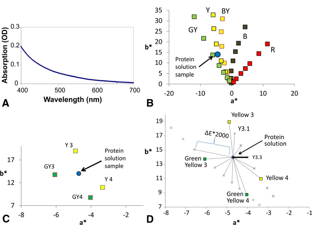
The quantitative spectral method requires three steps: (1) obtain an absorption spectrum of protein solution test sample as depicted in Figure 3A; (2) transform the absorption spectrum to the L*a*b* color space as shown in Figures 3B,C (9); and (3) within the L*a*b* color space, match the sample to the nearest reference color solution (Figure 3D).

Process of identifying best match (next darkest) in color series. (A) Take absorption spectrum of protein solution in 1 cm path length cuvette. (B) Convert absorption spectrum to L*a*b* values as described in the text. Plotted here is the protein sample in the a*b* plane. Notes: (1) All calculations are completed using three-dimensional L*a*b* space; plots only show a*b* plane for illustrative purposes. (2) The position of protein sample was chosen for illustration purposes; it is not the actual a*b* values derived from the absorption spectrum shown in plot 3A. (C) Enlarged plot of a*b* plane showing protein sample between green yellow (GY) and yellow (Y) color series. (D) a*b* plot showing protein color (blue), reference color solutions (squares), and interpolated points (x). Within three-dimensional space L*a*b* the ΔE2000 is calculated to both reference color solutions and interpolated points. The shortest distance gives best match, in this case Y3.3. The next-darkest readout is the next reference color solution within this color series, in this case Y3.
Although we follow colorimetric norms for transforming absorption spectrum to L*a*b* color space and also to calculate color-matching distances (ΔE2000), we have adapted the color-matching algorithm to closely correlate to the visual assessment method currently employed. To describe this algorithm, for simplicity we are again only showing the a*b* plane; however, all transformations and distances calculated involve the three-dimensional L*a*b* color space. For the example shown in Figure 3A–D, the protein solution color (after transformation to L*a*b*) falls between the Y and GY color series. In the visual assessment method, the analyst would then pick the reference color series of choice by picking a series that most closely matches the “color” or hue of the sample. If this is mathematically performed by measuring the distances from the protein sample to each reference color, the shortest line would be from the protein sample to GY3. As evident from the plot, the protein sample is actually closest to the yellow color series. The issue is that within the plot, the chromas of the color series are not aligned (GY4 and Y4 are not the same distance from water), and hence, assignment of the color series could be misleading.
In order to avoid this issue, we mathematically interpolate multiple points between measured adjacent Ph. Eur. color reference solutions within a color series (Figure 3C,D). This would be equivalent to increasing the number of dilutions within a color series. The ΔE2000 distance is then measured between the protein sample and the interpolated points (Figure 3C). The shortest distance allows for assignment of the color series (typically the color series with the hue closest to that of the test sample hue). Once a color series is selected, the analyst would then pick the next more intense reference color solution within the same color series. Within the a*b* plane, the more intense reference color solution is defined as having a larger chroma or further from water. In this case, we mathematically search for the next darker in the yellow color series, which is Y3 (Figure 3D). By following this procedure, as described later, we have demonstrated that one can correlate the visual assessment to a quantitative method. As such, the software reports a calculated value (closest interpolated point) and a report value (reference color solution).
Software Rules To Match the Visual Assessment Method
In addition to the above algorithm, we have implemented software rules such that solution colors (e.g., blue) that are not close to the color reference solutions or color intensities that are much more intense than the Ph. Eur. reference solutions are reported as not matching the Ph. Eur. reference solutions. This is important because the software should not always readout a best match independent of the actual solution's color. Below is a description of the algorithm rules that are shown visually in Figure 4.

Visualization of software rules employed, such that visual assessment matches current practices used in clinical laboratories conforming to the guidelines of GMP. White space is reported as “not reportable to Ph. Eur. color series”. See the text for description of software rules.
Samples within C* (Euclidean distance between points in a*b* plane) (2) of <0.25 of water a*b* (0, 0) and 99.00 < L <101.00 are reported as water (samples can have a negative b* if they are close to water, within experimental error). It should be noted the additional limit on L* values was implemented to detect improper standardization with air instead of water. In such cases the L* value for the initial water standard would report at values of approximately 102. With the limits on the L* value described above, that initial water standard sample would fail to read as water, which would prompt the analyst to re-standardize properly before reading samples.
Samples with a negative b* (not within a C* of 0.25 of water) are reported as not reportable to Ph. Eur. color series.
Currently it is our company practice when using the visual assessment method to report samples with a low amount of color to the B color series. As such, samples with a positive b* and chroma less than 1.19 (R7 chroma) are reported to the B color series.
Samples with a positive b* and chroma between 1.19 (R7 chroma) and 2.78 (B6 chroma) are reported to the closest match.
Samples with a positive b* and a hue above 131.6 (represented as degrees/angle in a*b* plane) or hue below 23.6 and with chroma greater than 2.78 (B6 chroma) are reported as not reportable to a Ph. Eur. reference color. These hue numbers were determined by allowing the hue to drift past the R series equal to half the hue distance between R and B series (at the maximum difference). The maximum allowed hue on the GY series side was determined by allowing color to drift past the GY series equal to half the greatest distance between the Y and GY series (at the maximum difference).
For samples that fall within the hue boundaries (described above in rule 5) but with chroma equal to or greater than R1, B1, BY1, Y1, GY1 (intensely colored) will read out as not reportable to reference color solutions (i.e., if calculated comes out as R1.0, B1.0, BY1.0, Y1.0, or GY1.0, the readout is not reportable to Ph. Eur. reference color solutions).
Although in the above cases the solutions are not reported as matching to a Ph. Eur. reference color, the L*a*b* values are still measured and recorded. In this manner, lot-to-lot variability of the solutions can still be tracked using their L*a*b* values. This allows for color release testing of protein solutions that do not fall within a yellow to slightly red hue covered by the Ph. Eur. color reference solutions.
Comparison of Quantitative Spectral Method to Visual Assessment Method
To demonstrate the correlation between the visual assessment method and the quantitative spectral method we have applied both techniques to the measurement of 15 protein solutions. We used selected monoclonal antibody (mAb) solutions that range from low to high concentration (20 mg/mL to 150 mg/mL), a range of turbidities (Ref I–Ref IV), and a range of color intensities (chroma) (Table VI). Each sample was assessed visually by five analysts; the same five analysts then performed the color assessment using the quantitative spectral method. For the visual assessment method, the same lot of reference color solutions was used for all analysts, thereby eliminating any variability in the determined color caused by the preparation of the reference colors and allowing for a direct comparison of the two methods. Prior to analysts selecting the best match of each protein sample to reference color solutions, the analysts were given a blinded set of reference color solutions and asked to match to reference color solutions. Without mistake the analysts and quantitative spectral method always correctly matched the test reference color solution to the actual reference color solution (11), demonstrating that the analyst could correctly choose the best match reference color solutions when the test solution exactly matched one of the reference color solutions. Although there are no protein solution samples with GY color, this comparative study between visual assessment and the quantitative method confirmed agreement between both methods for all color reference solutions (11).
Comparison of Visual Assessment to the Quantitative Spectral Method
Table VI compares the test results for the protein solutions from the visual assessment method and the quantitative spectral method. The quantitative spectral method demonstrates extremely reproducible results. In contrast to the quantitative method, the visual assessment method shows variability among the five analysts. For a given protein solution, different analysts reported different levels (intensity) of the same color series or in some cases reported adjacent color series. There was no clear trending correlating visual assessment variability to protein concentration or turbidity. It should be noted that most of these protein solutions, unlike the aforementioned study with reference color solutions, do not exactly match any reference color solutions and fall in between two reference color series, making it difficult for the different analysts to pick a consistent color series. To illustrate this point we have calculated the ΔE2000 values between the protein solutions (measured L*a*b* values) and the reference color solutions (L*a*b* values). As a reminder, following the visual test procedure outlined previously the analyst first compares the protein sample to all 37 reference color solutions and picks the closest match. The reference series that the best match belongs to is then assigned the color series of choice, and the analyst then picks the next most intense reference color solution in this series as the reported value. Following this procedure for sample #1 (Table VI), the closest reference color solution to the protein sample is B7 with a ΔE2000 = 0.6 (Appendix Table S4); the second closest match is BY7 with a ΔE2000 = 0.9. As mentioned previously, for most analysts a ΔE2000 = 0.5 is not a noticeable difference in color and a ΔE2000 = 1 is a just noticeable difference in color. So for this case it is difficult for the analyst to assign either the B or BY color series, hence resulting in four analysts choosing B and one choosing BY. For all proteins tested we have calculated the ΔE2000 between the best match and second best match color series. As the Y series for some samples is not the first or second calculated match but nonetheless was chosen by analysts, we have included it in Appendix Table S4. In all cases the difference in color ΔE2000 between the sample and color series reported by the analyst is within a ΔE2000 < 2, which is a very small color change and may be perceived differently by different analysts. The instrument method completely removes this variability in perception.
We were interested in cases where analysts chose Y as the color series and to understand the slight hue bias between the two methods. We hypothesized that a cause of differences between the visual assessment and quantitative assessment may be attributed to light scattering. For the visual assessment, the analyst looks down the long path length of the test sample (40 mm). As these protein samples do scatter light, some ambient light enters the sample tubes from the sides, and it will be scattered in a wavelength-dependent manner toward the observer, thereby changing the apparent visual color.
To test the impact of light scattering on the visual assessment of the protein solutions, we wrapped the sides of the test tubes with aluminum foil and re-evaluated the samples. Analysts noted that wrapping the tubes in foil did change the observed color. In some cases this resulted in a different reported color value as compared with unwrapped tubes (Table VII), indicating that light scattering contributes to the reported color values. After wrapping the tubes, all reported values were in the same or adjacent color series. In totality this data points to the potential variability of the current visual assay where analysts attempt to pick a best match between colors that do not match well. Factors such as the light source and how the analyst holds the sample tube (perhaps blocking ambient light entering the side of tubes) can contribute to the variability of the visual method. Frequently this variability is not observed in testing labs, as samples are only tested against the specified color series. This study highlights the impact that variables such as observation path length, stray light, temperature, and preparation reagents can have on the reported color.
Comparison of Visual Assessment Method with Sample Tube Wrapped in Aluminum Foil Compared with Sample Tube Not Wrapped in Aluminum Foil
Minor differences in the absolute color assignment between the visual method and the spectral method are more than compensated for by the greatly improved precision of the spectral method. The increased precision allows for a much more sensitive method for detecting batch-to-batch variability in color within a given process as well as changes in color that might occur as development proceeds and a manufacturing process changes during development, for example, Toxicology lot versus Phase I/II good manufacturing practice (GMP) lots versus Phase III and commercial GMP lots. It also allows for more accurate assessment of color changes that may occur in a given lot during stability studies.
Conclusion
We have described here a quantitative method for measuring and reporting a protein solution's color to Ph. Eur. reference colors. At low concentrations of therapeutic proteins, most solutions are close to colorless (colorless to barely perceptible color), and such a visual assessment of color may be sufficient. As an increasing number of therapeutic proteins are formulated at high concentrations, color intensities are certain to be higher. These more-colored solutions, especially the ones that fall between reference color series, can yield variable results with the visual assessment method. The quantitative spectral method allows for precise tracking of lot-to-lot variability of color solutions. We believe this method is comparable to the current visual assessment method and suitable for use in a QC laboratory for lot release and stability testing; the data supporting its suitability were obtained in a separate study (11).
In this current work, we present the Ph. Eur. reference color as a readout of a protein solution's color. Due to the precision of the assay, and because reference color solutions at low chroma are closely spaced, it is possible for low color chroma (intensity) samples to jump color series from one sample to another with very minor changes in actual color. The quantitative spectral method may report color changes that are not readily discernable via visual assessment. This should be taken into consideration in setting acceptance criteria. One approach is that during early stages of development one could consider these low-intensity reference colors (GY7, Y7, BY7, B9, B8, B7, and R7) to be equivalent. Additionally, for more-intensely colored samples, the color may lie near the boundary of two color series. In that case readings may also jump color series from sample to sample with relatively little real change in color. Therefore, in early development, some allowance for readings in adjacent color series should be considered in setting acceptance criteria. Later in development, as more manufacturing experience is gained and with increased product knowledge, adjustments to the acceptance criterion are considered and implemented as appropriate. At the time of licensure, it is foreseeable that color specifications will be set according to the L*a*b* color space rather than the Ph. Eur. reference colors or similar color standards. The shape of this color space used to set acceptance criteria should be a topic of discussion by the industry and regulatory agencies.
Conflict of Interest Declaration
The authors declare that they have no competing interests.
Acknowledgements
We thank Charlie Wang for data collection. We appreciate the support of this project by Jamie Moore, Samir Sane, and Sarah Du.
Appendix
A Spectral Method for Color Quantitation of a Protein Drug Solution
Trevor E. Swartz, Jian Yin, Thomas W. Patapoff, Travis Horst, Sue Skieresz, Gordon Leggett, Kimia Rahimi, Joseph Marhoul, and Bruce Kabakoff
Temperature Effect on Ph. Eur. Reference Color Solutions
%HCl Effect on Primary Color Solutions
Interpolated L*a*b* Points Used for Color Best Match
Comparison of Quantitative Color Match to Visual Assessment

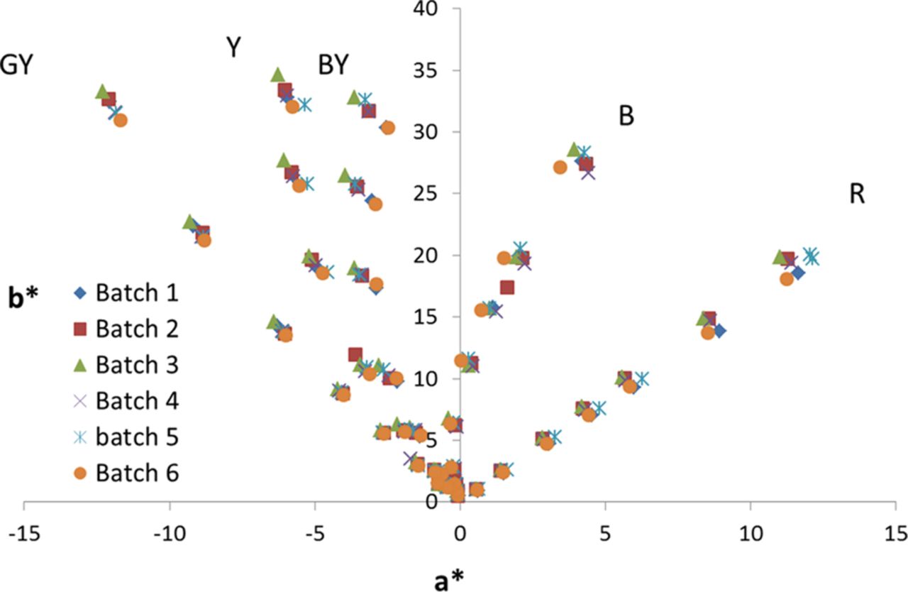
a*b* plot of six independently prepared batches of Ph. Eur. reference color solutions. Variability from prep to prep due to the “pipetting error” caused by volumetric preparation.

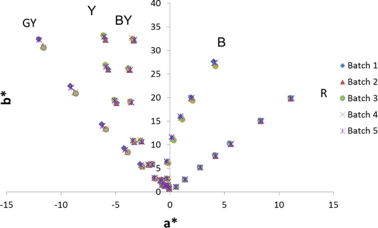
a*b* plot of six independently gravimetrically prepared batches of Ph. Eur. reference color solutions. Variability from preparation to preparation due to weighing is significantly less than the “pipetting error” caused by volumetric preparation.
- © PDA, Inc. 2016


