
Abstract
Due to the comparative nature of a bioassay, the relative potency is usually used to describe the potency of a sample. Only when the two samples are similar can a valid and meaningful estimate of relative potency be obtained. Thus, assessing similarity is a crucial part in developing a bioanalytical method. The current commonly used approach for assessing similarity focuses on the response parameters, such as the slope in the linear case, using either a significance test or an equivalence test. The current direct evaluation of the response parameters ignores the information about the shape of the curve and the possible variance heterogeneity. To overcome this, we propose a method based on the idea of equivalence testing that compares the shapes of the curves directly. The new method first measures the difference of the response between the standard sample and the test sample at each of the concentration (dilution) levels and then determines whether the differences are consistent by comparing them to the equivalence limits. The benefits of the new method are investigated by a simulation study.
LAY ABSTRACT: Due to the comparative nature of a bioassay, the relative potency is usually used to describe the potency of a sample. Only when the two samples are similar can a valid and meaningful estimate of relative potency be obtained. Thus, assessing similarity is a crucial part in developing a bioanalytical method. The current commonly used approach for assessing similarity focuses on the response parameters, such as the slope in the linear case, which have many drawbacks To overcome this, we propose a method based on the idea of equivalence test but comparing the shape of curve directly. The new method first measures the difference of the response between the standard sample and the test sample at each of the concentration (dilution) levels and then determines whether the differences are consistent by comparing them to the equivalence limit.
- Bioassay
- Relative potency
- Similarity
- Parallelism
- Equivalence limits
- Difference
- Shape of curve
- Capability limits
- Fixed limits
1. Introduction
Bioassays are critical in developing biological products and vaccine. Due to the comparative nature of a bioassay, the estimated potency of the test sample is usually expressed in terms of the relative potency (RP) with respect to a standard preparation. The RP is determined as the ratio between doses that achieve equal mean responses of the test and the standard to the stimulus (1). It is a singular measure of how much the test preparation should be diluted (or concentrated) to get the same potency as the standard preparation (2). For this RP to be meaningful, the test preparation must behave as a dilution (or concentration) of the standard preparation. In the literature, this is often referred to as similarity or, more colloquially, as parallelism. Without an assurance of similarity, the investigator would not be able to derive a reliable and meaningful relative potency. Evaluating similarity is thus a critical step in developing bioanalytical methods for measuring potency.
Mathematically, similarity can be defined as two curve functions having the following relationship (Finney, 1978): f1(x) = f2(ρx) where f1 represents the dilution function for the test preparation, f2 represents the dilution function for the standard preparation, x is the concentration/dilution level, and ρ is the relative potency. When two curves are similar and the response is plotted against the logarithm of dilution (or concentration), the test preparation curve will have exactly the same shape as the standard preparation curve but horizontally shifted. The amount of shift is the logarithm of relative potency. It is clear that two linear curves are similar if and only if they have the same slope. In this paper, we mainly focus our discussion on the linear case.
To assess similarity, the traditional approach uses a statistical hypothesis test to justify whether the slopes are equal. Lack of statistical significance at a certain predetermined level is taken as an indication of similarity. The shortcomings of this counterintuitive approach are well documented. In particular, as described in Hauck et al. (3), increasing the precision of the assay may lead to frequent rejections of runs that exhibit only minor departures from parallelism. In contrast, for an assay with poor precision, this approach may conclude similarity even when the test sample is clearly not parallel to the standard. This problem stems from the formulation of the null hypothesis as the hypothesis of similarity, the hypothesis the laboratory wants to accept. This is counter to scientific studies where the null hypothesis is taken to be the status quo, the hypothesis that is assumed until sufficient evidence is obtained to support its rejection. Proving similarity (i.e., assuming dissimilarity) is the proper scientific strategy, not the other way around.
Because the goal is to determine if the two samples are sufficiently similar rather than to prove that the difference is significant, it would be better to start with the correct alternative hypothesis (H1). This is why equivalence testing has been considered and proposed to replace the classical significance test in the revised USP Chapter 〈111〉. In fact, Hauck et al. (4) stated that in the revised USP Chapter 〈111〉, the test for parallelism will be based on an equivalence testing approach, and the current hypothesis testing approach will no longer be acceptable for determining similarity. Equivalence testing argues that a certain degree of nonsimilarity is acceptable in the sense that such departures from parallelism have no meaningful impact on results obtained or decisions made on unknown test samples. Methods for determining this acceptable degree of nonparallelism have been considerably discussed in the linear case (3, 5). In general, these fall into one of the two categories: (1) Fixed limits, based on historical data or scientific judgment, and (2) Capability limits, based on comparing the standard preparation to itself over many runs. The first case controls the false passing similarity. The latter case controls the false failing similarity. Thus, any difference in slopes, for example, must be attributed to assay variability and not some kind of “matrix effect.”
The dilution effect (DE) is an index introduced in the industry to assess dilution similarity (6) by measuring the percent bias per, say, 2-fold dilution in a test sample's value relative to that of the reference standard. It is defined as follows.
 where bT and bS are the estimated slopes for the test and the standard, respectively. A dilution effect less than 20% in absolute value has been used in industry to conclude dilution similarity or parallelism. While the use of this index is simple and convenient, it does not take the variability in the data into consideration and may lead to different conclusions if the plate positions of the test sample and the standard sample are switched. A DE of 20% might be acceptable for an assay using five twofold dilutions ranging from 1:2 to 1:32 but unacceptable for an assay using five fourfold dilutions ranging from 1:2 to 1:384. Thus, using this index for a formal similarity assessment should be done cautiously.
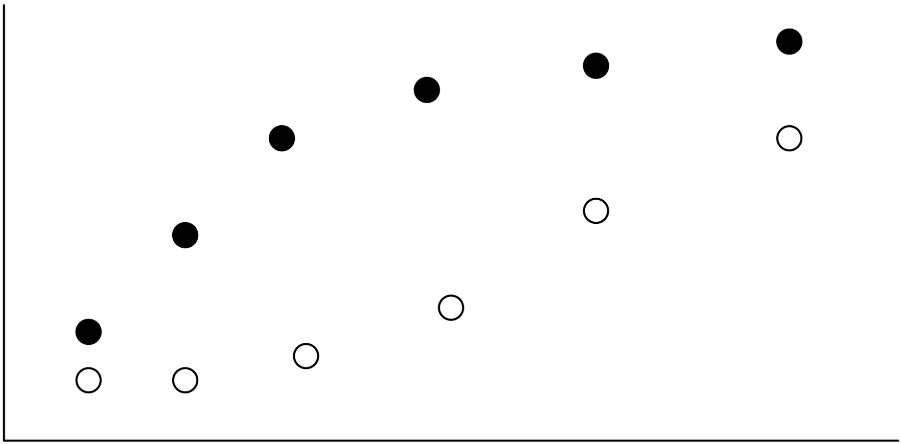
In the literature, similarity assessments have focused only on comparing two slopes, rather than comparing the shape of the two curves. While this is sensible, it is difficult to determine how much of a difference is acceptable because the slope is not directly linked to the raw data; it is only a summary of them. For example, the use of 20% for the DE is based on experience more than any direct impact such a departure from parallelism has on the quality of the data obtained on an unknown test sample. A subject matter expert may be more readily able to define (and defend) what constitutes an acceptable difference in assay response compared to what constitutes an acceptable difference in slopes. This problem is even more pronounced when more than one parameter needs to be evaluated to assess similarity, as in the case of many nonlinear models, due to the complex joint parameter region (7, 8). Another drawback to focusing on the slopes only can be seen in Figure 1, where the focus only on slope overlooked the possible curvature and the variance heterogeneity at each concentration level. In this figure, there is a perfect similarity based on comparing the slopes, but the true curves are clearly nonsimilar.

The difference between the slope focus and the curve shape focus.
In Section 2, we propose a new method that directly measures the difference of the curve shape. Instead of setting up a limit for the slope difference, we establish the equivalence limit for the difference of the shape for the whole curve. Instead of using only one type of interval, the equivalence limits recommended are the joint region of a fixed interval and the capability-based interval to balance the false passing similarity and false failing similarity rate. In Section 3, the results from a simulation study are presented and show the advantage of the proposed method. Section 4 summarizes our findings.
2. The New Method
The basic idea of similarity has been summarized as “we assume that the standard preparation contains no substance, other than factor X itself, contributing to the response we measure and that the test preparation behaves as for the purpose of analysis so similarly to the standard preparation that it may be regarded simply as a dilution of the standard preparation in a completely inert diluent” (9). Before introducing the new method, the mathematical notations for the rest of the paper are summarized in Table I .
Mathematical Notations Used in This Paper
In a typical linear assay, the logarithm of the mean response is usually a linear function of the logarithm of the concentration, that is,
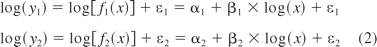 where y1 and y2 are the responses for the test sample and the standard sample, respectively, and x represents the level of concentration, α1 and β1 are the intercept and slope for the test sample, α2 and β2 are the same for the standard, and ε1 and ε2 are the normally distributed residual errors (with mean 0 and constant variance σ2) corresponding to the test and standard preparations, respectively. The heterogeneous variance case will be discussed later.
It is straightforward to show that two linear curves are similar (i.e., β1 = β2 = β) if and only if E[log(y1)] − E[log(y2)] = β × log(ρ) = α1 − α2 = C, for all concentration or dilution levels. This equality means that for any concentration or dilution level x, the difference between the logarithm of test preparation and standard preparation is a constant C. Under similarity, then, the logarithm of relative potency (log(ρ)) is (α1 − α2)/β = C/β. As a consequence, determining the similarity between two linear preparations is equivalent to determining whether the difference of response is consistent over all concentration levels.
Let I be the dilution levels with corresponding concentrations: x1, x2, … xi … xI, and J be the replications at each dilution level. Thus at dilution level i, the responses are yi1, yi2 … yij … yiJ The observations of response are considered mutually independent. An example data structure is provided in Table II for J = 3, I = 5. In this case, the sample size n = 2 × I × J = 30.
Data Structure
Since both log(y1ij) and log(y2ij) have a normal distribution, log(y1ij) − log(y2ij) = δ1 + ε1ij − ε2ij = δi + ηij has a normal distribution with mean δi = α1 − α2 − (β1 − β2)log(xi) and variance 2σ2, which is a perfect one-way analysis of variance (ANOVA) setting for a factor with I levels. If the underlying true curves are linear and they are similar, then δ1 = δ2 = … = δl = βlog(ρ) = C. Therefore, assessing similarity in the linear case is equivalent to assessing the condition
 To accomplish this in a scientifically acceptable manner, we conduct the equivalence test as defined in eq 4 below
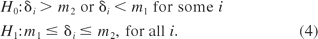 The first step is to determine the equivalence interval [m1, m2] then obtain the confidence interval for each δi. If all of the confidence intervals fall entirely within the equivalence interval, then we conclude H1 and therefore that the two samples are similar.
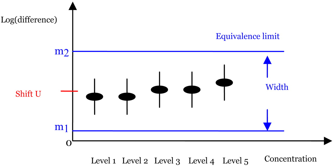
The idea of the new method is illustrated in Figure 2 with five concentration levels. In this figure, the black solid dots represent the estimates of δi, the difference in log-responses. The vertical black solid lines are the corresponding confidence intervals. The two blue horizontal dotted lines are the pre-determined equivalence limits. Note that the equivalence limits in this figure are not centered at 0. The center of the equivalence limit is shifted by a constant, U. The determination of U will be discussed later along with the determination of the equivalence limits. Since all of the confidence intervals fall within two horizontal blue dotted lines in this figure, we conclude that the two samples are similar. Figure 2 reveals the advantages of the new method, including capturing the patterns of the differences and the possible nonhomogenous variance among the concentration levels.

Graphical illustration of the new method for five concentration levels.
2.1. Obtaining the Confidence Intervals for δi
To determine the confidence interval for δi, which is the mean of log(y1ij) − log(y2ij), we first calculate the difference of the logarithm of the responses, and then do an ANOVA on these differences as in the model log(y1ij) − log(y2ij) = δi + ε1ij − ε2ij = δi + ηij where ηij has a normal distributed with mean 0 and variance 2σ2. From the ANOVA, the estimate of δi and its estimated variance Var(δi) can be easily obtained. Thus the 95% approximate confidence interval of δi is
2.2. Constructing the Equivalence Limit
The width of the equivalence limit:
The width of the equivalence limit represents the maximum distance that a nonparallelism can be practically considered as acceptable. Accepting any level of nonparallelism is an acceptance of bias in the measurement of relative potency. If we have prior knowledge that, for example, relates the level of bias in the assay measurement to clinical or other scientific outcomes, the equivalence limit should be established based on that information. However, this kind of information is generally not available nor easy to obtain, especially in the early development stage.
In lieu of such prior information, we recommend constructing the equivalence interval as a type of tolerance interval based on collecting data from R multiple independent experimental runs consisting of assaying the standard (or control) preparation against itself. In this experiment, because the standard is similar to itself, a series of confidence intervals and a series of corresponding widths can be obtained. Those widths for the 95% confidence interval show the possible range of
If it is not feasible, which is usually the case in practice, to perform a series of “standard vs standard” experiments to estimate Var(δ̂r), which is a multiple of σ2, we recommend using the data from the standard preparation only to estimate variance σ̂ to form the tolerance limits. Assume the amount of shifting is U, the capability based limit could be calculated as
The amount of shift—U:
As discussed earlier, two linear preparations are similar if and only if there exists a ρ such that E[log(y1)] − E[log(y2)] = β × log(ρ) = α1 − α2 = C, for all concentration or dilution levels. The amount of shifting U represents the difference of logarithm of response when there is no random error. When the preparations are similar, then U = E[log(y1)] − E[log(y2)] = β × log(ρ) = α1 − α2 = C.
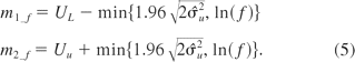
The common problem of a capability- or tolerance-based strategy is that the intervals may be unacceptable wide because this type of interval controls the false failing similarity rate, not the false passing similarity rate. This usually happens in an assay with poor precision. Some modifications to the equivalence intervals are needed to prevent this constructing such intervals based on using data when we have a highly variable assay. Recall at Section 1, the equivalence interval is introduced as a measure for the variation of confidence intervals of δi, the expectation of log(y1ij) − log(y2ij). The wider the equivalence interval, the more likely this test concludes similarity, even for a highly variable assay. Thus, we need to have a fixed limit to control the false passing similarity rate. If we have information that beyond a certain fold difference, for example, a 2-fold or 3-fold difference, similarity is not acceptable from a practical point of view, and then we should incorporate that information in our decision making process. In general, an f-fold boundary is of the form where f = 2 or f = 3 are common choices. To incorporate this information, the equivalence interval can be expressed as (m1_f, m2_f), where
 The equivalence interval defined in eq 5 is the joint region of a fixed limit controlling the false passing similarity and a capability-based interval controlling the false failing similarity, and it balances the false passing similarity rate and the false failing similarity rate.
3. Numerical Comparison
To illustrate the advantage of the new approach, several simulation studies were conducted. In the simulation studies, the new method was compared with the DE index and the F test. J was used to represent the new method just described above without a fixed limit, J2 was used to represent the new method with a 2-fold boundary (f = 2), and J3 was used to represent the new method with a 3-fold boundary (f = 3).
The data were simulated based on eq 6 below. A 2-fold serial dilution was used to generate concentration levels from 16 to 1 units, that is, log(x) = log(1), log(2), log(4), log(8), log(16). Without loss of generality, the intercepts for both the test preparation and the standard preparation were fixed as a1 = a2 = 1. Different slopes were used where β2 = 1 vs β1 =1, 1.01, 1.1, 1.3, 1.5, and 2. Suppose when β1 ≤ 1.1 the two linear curves are considered acceptably parallel and when β1 ≥ 1.5 the two linear curves are not considered acceptably parallel. To investigate the impact that the residual variance (σ2) has on the methods, different relative standard deviation (RSD) levels were used in the simulation: RSD = 10%, 20%, 30%, 50%, and 100%. At each concentration level, three independent observations were simulated.
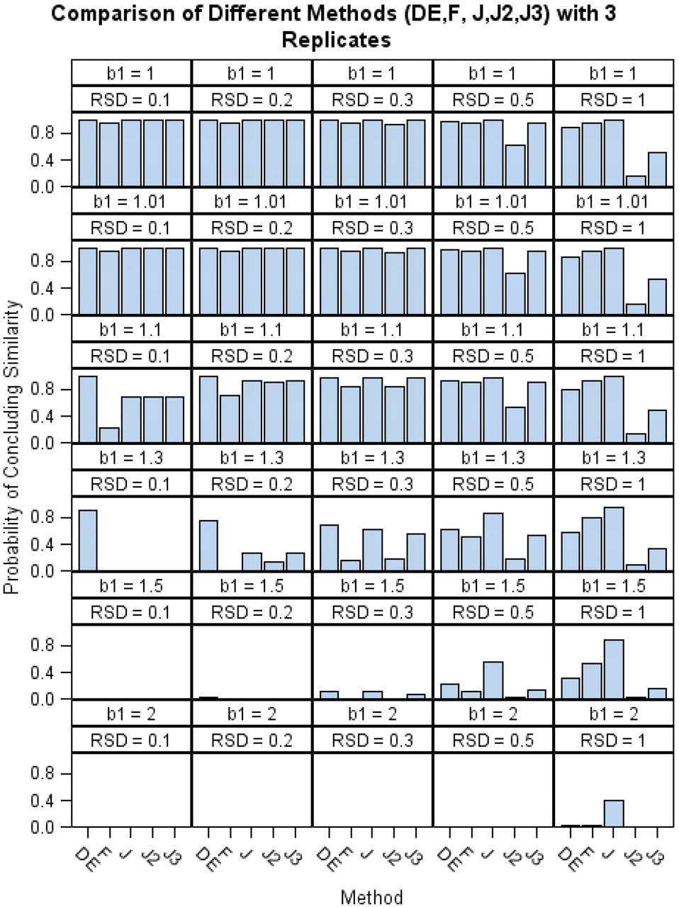
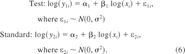 Figure 3 summarizes the percentages of concluding similarity (y-axis) for each method among 1000 simulations in all 30 combined scenarios. There are five vertical panels representing the five different RSDs for each of the six different slope levels in the figure. For each method, the higher the bar is, the more likely a method is to conclude similarity. In the first scenario (β1 = 1), the two preparations are identical; thus they are perfectly similar. When the RSD is small, all of the methods are able to make the correct conclusion. As shown in the figure, J, J2, and J3 methods produce very close percentages due to the fact that the practical 2-fold or 3-fold fixed boundaries do not have any impact on the equivalence interval for an assay with small variation. However, when the RSD is large, for example, when RSD is 100%, a dramatic drop is shown at J2 and J3. This can be viewed as penalizing assays with poor precision by controlling the false passing similarity rate. In the second and third scenarios, the two curves are not exactly similar: β1 ≤ 1.1, but practically, this difference is considered acceptable. When the RSD decreases from 100% to 10%, the likelihood of concluding similarity using the F test decreases from 94.1% to 22.4%. This shows that very precise data can lead to the rejection of the similarity hypothesis even if the difference is considered minor. In the fourth scenario, the two curves are not similar, but not too dissimilar either (β1 = 1.3). In this case, all methods except the DE are able to make the correct “dissimilar” conclusion when the RSD is small. For large RSDs, the J2 and J3 methods generated the greatest chance of correctly concluding nonparallelism. In the last two scenarios, the two curves are not similar: β1 ≥ 1.5. When the variation is small, there are no bars in the picture, as all of the methods correctly conclude the two curves are not parallel. However, when the variation is high, most of methods have trouble rejecting the similarity except J2 and J3.

Numerical comparison of the different methods.
In conclusion, from the simulation studies, the proposed method performs very well and provides advantages over existing approaches. The joint equivalence region from both the capability-based interval and the fixed limit should be used to control and balance the false failing similarity and false passing similarity rate.
4. Summary and Discussion
Similarity is a requirement for the estimation of relative potency. In this paper, we proposed a methodology to assess similarity based on the idea of equivalence testing using the difference of two responses at the same concentration level instead of the curve parameters, such as the slope in the linear case. This new method assesses the difference of curve shape directly. The advantages of the new method are (1) capturing dilutional trends resulting from “matrix effects,” (2) identifying nonhomogenous variability among the concentration levels, and (3) controlling the rate of falsely claiming nonsimilarity with incorporating any clinical or practical subject knowledge into consideration to control false passing similarity. In addition, this method is very easy to apply with common commercial software, such as SAS® or Minitab®. The simulation studies indicate that the new method with a 2-fold boundary or a 3-fold boundary (J2, J3) performs better than the other methods in regards to sensitivity and specificity and thus the joint equivalence region from both the capability-based interval and the fixed limit is recommended for use to control and balance the false failing similarity and false passing similarity rate.
We have focused on the linear case in this paper. However, the proposed approach can be also modified to assess the similarity for a nonlinear response curves such as the four-parameter logistic or the five-parameter logistic functions. This will be presented in detail in a separate paper.
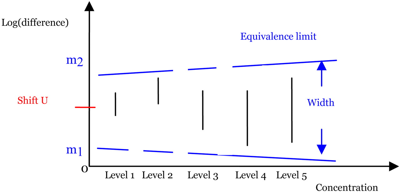
Up to this point, we assumed that the residual variance was homogeneous. However, the new method can easily be modified to handle the heterogeneous variance case. For example, suppose the variance is a power function of the logarithm of the response: Var(log(y)) = σ2log(y)θ, where σ2 and θ are unknown parameters. Conceptually, assessing similarity in the heterogeneous variance case is the same as that in homogeneous variance case. Now, the difference in log responses, log(y1ij) − log(y2ij), has a normal distribution with a nonconstant variance σ2 · [log(y1)θ + log(y2)θ]. Using SAS® procedure NLMIXED (10), an analysis similar to an ANOVA can be performed to obtain the confidence interval for the difference δi (i = 1 to I) at each concentration level. However, the equivalence interval is not constant over the entire concentration range but is instead an “equivalence curve” because the variance is response-dependent variance. The greater the response, the wider the equivalence interval, as shown in Figure 4, where the blue dashed lines represent the equivalence curves. If all of the confidence intervals fall entirely within the equivalence curves, then similarity is claimed.

Graphical illustration of the new method for five concentration levels in the heterogeneous residual variance case.
Conflict of Interest Declaration
There is nonfinancial competing interest related to the paper.
Acknowledgements
The authors thank the editor and two referees for their valuable comments that improved the presentation of this paper.
- ©PDA, Inc. 2011


